Introduction
In the rapidly evolving world of artificial intelligence, the deployment of powerful neural networks into real-world applications often hits a bottleneck: their immense computational and memory requirements. AI model quantization is a critical optimization technique designed to address this challenge. It allows large, complex models—trained using high-precision floating-point numbers—to be compressed and executed efficiently on resource-constrained devices, from smartphones and IoT sensors to specialized AI accelerators.
Understanding the internals of quantization is no longer a niche skill but a fundamental requirement for AI engineers and researchers aiming to build performant and deployable AI systems. It bridges the gap between theoretical model development and practical application, enabling faster inference times, reduced memory footprints, and lower power consumption.
This guide will provide an in-depth explanation of AI model quantization, drawing a powerful and intuitive analogy to sound recording and audio quantization. We will explore the core principles from first principles, dissecting how continuous signals translate into discrete representations, and then directly mapping these concepts to the weights and activations within neural networks. By the end, you will possess a deep, intuitive understanding of quantization, its mechanisms, trade-offs, and practical implications, ensuring this complex concept becomes clear and unforgettable.
The Problem It Solves
Modern AI models, especially deep neural networks, are often trained using 32-bit floating-point numbers (FP32) for their weights and activations. This high precision offers a vast dynamic range and fine granularity, which is crucial during the iterative optimization process of training. However, this comes at a significant cost:
- Large Memory Footprint: Each FP32 number occupies 4 bytes. A model with millions or billions of parameters quickly consumes gigabytes of memory, making deployment on devices with limited RAM challenging.
- High Computational Cost: Floating-point arithmetic, especially 32-bit operations, is computationally intensive. It requires more complex circuitry and consumes more power compared to integer arithmetic. This translates to slower inference speeds and higher energy consumption.
- Deployment Challenges: Edge devices (e.g., embedded systems, mobile phones, smart cameras) often lack the powerful GPUs and ample memory found in data centers. Deploying large FP32 models on these devices is often infeasible due to latency, power, and memory constraints.
The core problem quantization solves is transforming these resource-hungry FP32 models into more compact and computationally efficient forms, typically using lower-bit integer representations (e.g., INT8, INT4), without significant loss in model accuracy.
High-Level Architecture
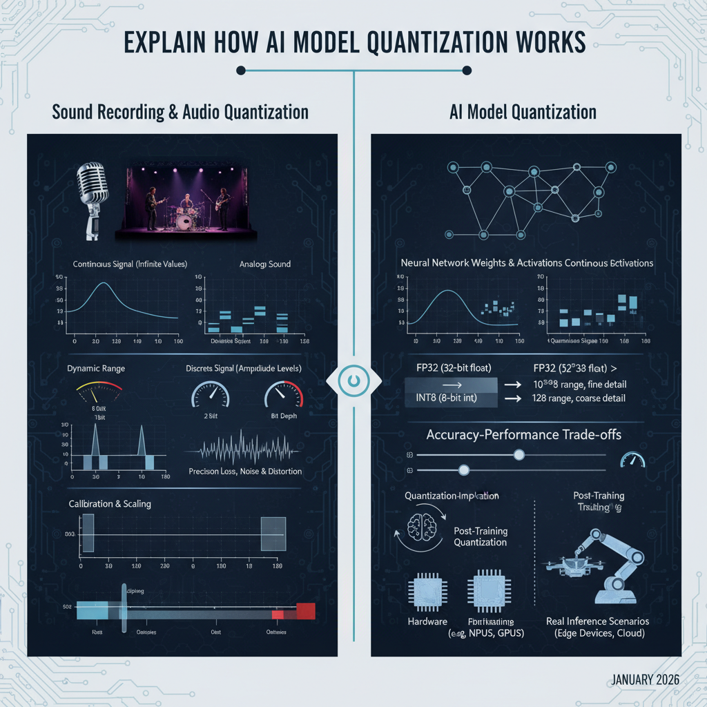
To grasp AI model quantization, let’s first establish a strong analogy with audio quantization. Imagine recording a live musical performance.
An analog sound wave is a continuous signal, varying smoothly in amplitude over time. To store or transmit this sound digitally, we must convert it into a discrete format. This involves two main steps: sampling (discretizing time) and quantization (discretizing amplitude).
In audio, an Analog-to-Digital Converter (ADC) performs this task. It takes snapshots of the continuous waveform at regular intervals (sampling) and then maps the amplitude of each snapshot to the nearest discrete level from a predefined set (quantization). The number of levels available depends on the “bit depth” (e.g., 16-bit audio offers 65,536 distinct amplitude levels).
Now, let’s map this directly to AI models:
- Continuous Analog Signal: This is analogous to the high-precision FP32 weights and activations within a trained neural network. These values can theoretically take on any value within their range, much like a continuous sound wave.
- Sampling: In AI quantization, we are not discretizing time, but rather the values themselves. The “samples” are the individual FP32 weights and activation values.
- Quantization: This is the core process where we map these continuous-range FP32 values to a limited set of discrete integer values (e.g., INT8). This is like an ADC mapping continuous voltage levels to discrete digital numbers.
- Digital Representation: The resulting quantized integers (INT8, INT4) are the compact, efficient digital representation, similar to how digital audio files store discrete amplitude values.
The high-level architecture for AI model quantization therefore involves taking an existing FP32 model and applying a transformation process to convert its numerical representations.
Component Overview:
- FP32 Trained Model: The original, high-precision model resulting from training.
- Quantization Algorithm: The core logic that performs the transformation, including calibration steps.
- Calibration Data: A small, representative subset of the training or validation data used to observe the distribution of weights and activations, crucial for determining the mapping parameters.
- Quantized Model INT8: The output model, where weights and often activations are stored and processed using lower-bit integers.
- Inference Engine: Specialized runtime environments (e.g., TensorFlow Lite, ONNX Runtime) optimized to execute quantized models efficiently, often leveraging hardware accelerators.
- Output: The prediction or result from the quantized model inference.
How It Works: Step-by-Step Breakdown
Let’s break down the process of AI model quantization, weaving in our audio analogy at each step.
Step 1: Continuous vs. Discrete Signals - The Foundation
Audio Analogy: Imagine a musician playing a violin. The sound waves produced are continuous; their pitch and volume can vary infinitesimally. A microphone converts these physical vibrations into a continuous electrical voltage signal.
AI Model Context: Similarly, the weights (parameters) and activations (intermediate outputs) within a neural network are typically represented as FP32 numbers. These are “continuous” in the sense that they can represent a vast range of fractional values with high precision. For example, a weight could be 0.00123456789 or 0.00123456790.
Step 2: Bit Depth and Dynamic Range - Defining Precision and Span
Audio Analogy: To digitize the continuous electrical signal, an Analog-to-Digital Converter (ADC) first “samples” the voltage at regular intervals (e.g., 44,100 times per second for CD quality). Then, for each sample, it assigns a discrete numerical value from a limited set. The size of this set is determined by the “bit depth.”
- 16-bit audio: Allows for $2^{16} = 65,536$ distinct amplitude levels. This defines the dynamic range (the ratio of the loudest to the quietest sound it can represent).
- 8-bit audio: Only $2^8 = 256$ levels. Much smaller dynamic range, leading to noticeable “quantization noise” or “stair-stepping” if the original signal was high fidelity.
AI Model Context:
- FP32 (32-bit float): Offers immense dynamic range and precision (approximately 7-8 decimal digits of precision). It’s like a 64-bit or higher audio recording—lots of detail and range.
- INT8 (8-bit integer): Allows for $2^8 = 256$ distinct integer values. This is significantly less precise than FP32.
- INT4 (4-bit integer): Allows for $2^4 = 16$ distinct integer values. Even less precise.
The goal of quantization is to map the wide range of FP32 values into these much fewer INT8 or INT4 levels. This inherently involves precision loss, just like converting a high-fidelity audio recording to a low-bitrate format.
# Example: Illustrating bit depth difference
fp32_val = 0.00123456789  # High precision
print(f"FP32: {fp32_val}")

# Simplified concept of INT8 - mapping to an integer
# Actual mapping involves scale and zero_point, shown in next step
# For now, imagine a range of -128 to 127 or 0 to 255
# If we had a range of -1 to 1 mapped to -128 to 127
# A simplified mapping might look like:
int8_approx = int(fp32_val * 127) # This is NOT how it actually works, just for illustration
print(f"INT8 (simplified): {int8_approx}")
Step 3: The Quantization Process - Mapping Values
Audio Analogy: When an ADC quantizes an audio sample, it takes a continuous voltage reading (e.g., 0.735V) and maps it to the closest available digital level (e.g., if levels are 0.01V apart, it might map to 0.73V or 0.74V, represented by an integer like 73 or 74). This mapping involves a scale (how many volts per digital step) and a zero_point (where the 0V level maps to in the digital range).
AI Model Context: The core of AI model quantization is this mapping. For a given tensor (weights or activations), we need to determine a scale factor (S) and a zero_point (Z). These two parameters define how floating-point values are converted to integers and vice-versa.
The formula for quantizing a floating-point value $r$ to an integer $q$ is:
$q = \text{round}(r / S + Z)$
And to dequantize back to an approximate floating-point value $r’$:
$r’ = (q - Z) \times S$
- Scale (S): This factor determines the range of floating-point values that the integer range will cover. A larger scale means each integer step covers a wider range of floating-point values, sacrificing precision but increasing dynamic range.
- Zero Point (Z): This integer offset ensures that the floating-point value
0.0maps exactly to an integer value. This is crucial for handling biases and ensuring certain operations behave correctly. For unsigned INT8 (0 to 255), Z is typically around 128. For signed INT8 (-128 to 127), Z is often 0.
Example: Quantizing a float to unsigned INT8 (0 to 255) Assume we have a tensor whose values range from -1.0 to 1.0. We want to map this to the INT8 range of 0 to 255.
Determine S and Z:
min_float = -1.0,max_float = 1.0min_int = 0,max_int = 255S = (max_float - min_float) / (max_int - min_int) = (1.0 - (-1.0)) / (255 - 0) = 2.0 / 255 ≈ 0.007843Z = min_int - round(min_float / S) = 0 - round(-1.0 / 0.007843) = 0 - round(-127.5) = 0 - (-128) = 128(for unsigned INT8)
Quantize a value: Let
r = 0.5q = round(0.5 / 0.007843 + 128) = round(63.75 + 128) = round(191.75) = 192
Dequantize back: Let
q = 192r' = (192 - 128) * 0.007843 = 64 * 0.007843 ≈ 0.501952Notice the slight difference (0.501952vs0.5) due to precision loss.
# Example: Quantization function
def quantize_value(r_float, scale, zero_point, num_bits=8):
    q_min = 0
    q_max = (1 << num_bits) - 1 # For unsigned integers (0-255 for 8-bit)

    q_val = round(r_float / scale + zero_point)
    # Clip to the integer range
    q_val = max(q_min, min(q_max, int(q_val)))
    return q_val

def dequantize_value(q_int, scale, zero_point):
    return (q_int - zero_point) * scale

# Parameters from example
scale_val = 2.0 / 255
zero_point_val = 128

original_float = 0.5
quantized_int = quantize_value(original_float, scale_val, zero_point_val)
dequantized_float = dequantize_value(quantized_int, scale_val, zero_point_val)

print(f"Original FP32: {original_float}")
print(f"Quantized INT8: {quantized_int}")
print(f"Dequantized FP32: {dequantized_float}")
print(f"Error: {abs(original_float - dequantized_float)}")
Step 4: Quantized Operations and Inference
Audio Analogy: Once audio is digitized, operations like volume adjustment or mixing can be performed on the digital samples. For example, to double the volume, you might multiply each digital sample by 2. If the result exceeds the max bit depth, it “clips,” causing distortion.
AI Model Context: The real benefit of quantization comes during inference. Instead of performing FP32 multiplications and additions, the model performs INT8 operations. For example, a typical neural network operation is a matrix multiplication: $Y = W \times X + B$. If $W$, $X$, and $B$ are all quantized: $W_{float} \approx (W_{int} - Z_W) \times S_W$ $X_{float} \approx (X_{int} - Z_X) \times S_X$ $B_{float} \approx (B_{int} - Z_B) \times S_B$
Substituting these into the original equation: $Y_{float} \approx ((W_{int} - Z_W) \times S_W) \times ((X_{int} - Z_X) \times S_X) + ((B_{int} - Z_B) \times S_B)$ $Y_{float} \approx (W_{int} - Z_W) \times (X_{int} - Z_X) \times S_W \times S_X + (B_{int} - Z_B) \times S_B$
The key is that the integer multiplications $(W_{int} - Z_W) \times (X_{int} - Z_X)$ can be performed using efficient integer hardware instructions. The intermediate results of these integer products can often accumulate in a higher precision integer (e.g., INT32) to prevent overflow, before being rescaled back to INT8 for the next layer. This “quantize-dequantize” (or “QDQ”) pattern is common in quantized inference, effectively performing calculations in integer domain and only converting to float for the final output or specific sensitive operations.
Step 5: Calibration - Finding the Right Scales and Zero Points
Audio Analogy: Before recording a song, a sound engineer adjusts the input gain levels. Too high, and the audio “clips” (distorts) at loud parts. Too low, and the recorded signal is too quiet, and quantization noise becomes prominent. This level setting is analogous to calibration.
AI Model Context: Determining the optimal scale and zero_point for each tensor (weights and activations) is crucial for minimizing accuracy loss. This process is called calibration.
- Weights: Weights are static after training, so their
SandZcan be determined once by analyzing their distribution (e.g., min/max values). - Activations: Activations are dynamic, varying with each input. Therefore,
SandZfor activations are usually determined by running a small, representative dataset (calibration dataset) through the FP32 model and observing the actual min/max or histogram distribution of activations for each layer.
Common calibration methods for Post-Training Quantization (PTQ):
- Min-Max: Simplest. Finds the minimum and maximum observed values for a tensor and maps them to the full integer range. Sensitive to outliers.
- Histogram-based (e.g., KL Divergence): More robust. It collects histograms of activation distributions and then finds
SandZthat minimize the information loss (e.g., using Kullback-Leibler divergence) when mapping the FP32 distribution to the INT8 distribution. This often ignores outliers to preserve accuracy for the bulk of the values.
Deep Dive: Internal Mechanisms
Mechanism 1: FP32 vs. FP16 vs. INT8/INT4 Representations
At the heart of quantization is the fundamental difference in how numbers are represented in memory and processed by hardware.
| Feature | FP32 (Single-Precision Float) | FP16 (Half-Precision Float) | INT8 (8-bit Integer) | INT4 (4-bit Integer) |
|---|---|---|---|---|
| Bits | 32 | 16 | 8 | 4 |
| Memory/Number | 4 bytes | 2 bytes | 1 byte | 0.5 bytes (packed) |
| Structure | Sign (1) Exp (8) Mantissa (23) | Sign (1) Exp (5) Mantissa (10) | Fixed Point (Magnitude) | Fixed Point (Magnitude) |
| Approx. Range | $\pm 10^{38}$ | $\pm 65504$ | -128 to 127 (signed) or 0 to 255 (unsigned) | -8 to 7 (signed) or 0 to 15 (unsigned) |
| Approx. Precision | ~7 decimal digits | ~3-4 decimal digits | Fixed (e.g., scale factor) | Fixed (e.g., scale factor) |
| Dynamic Range | Very High | Medium | Limited (determined by scale) | Very Limited (determined by scale) |
| Hardware Support | Universal | Modern GPUs, AI Accelerators | Modern GPUs, AI Accelerators, CPUs (ARM NEON) | Specialized AI Accelerators |
| Analogy | Studio Master Recording | High-Quality FLAC/WAV | Good Quality MP3 | Low-Quality MP3/Voice Memo |
- Floating-Point (FP32, FP16): These formats use a sign bit, an exponent, and a mantissa (fraction) to represent numbers. This allows them to represent a very wide range of values (dynamic range) and maintain relative precision across that range. FP32 is the standard for training. FP16 offers a good balance for some inference scenarios, especially on GPUs.
- Integer (INT8, INT4): These formats simply represent whole numbers. Their range is fixed and limited (e.g., 256 unique values for INT8). To represent fractional values, they rely on the
scaleandzero_pointto implicitly define the decimal place. This is why they are often called “fixed-point” representations in this context. Integer arithmetic is significantly faster and more power-efficient on modern processors and specialized AI accelerators, which often have dedicated INT8 instruction sets.
import numpy as np

# Illustrating the range and precision differences
val_fp32 = np.finfo(np.float32)
val_fp16 = np.finfo(np.float16)

print(f"FP32: Min={val_fp32.min}, Max={val_fp32.max}, Epsilon={val_fp32.eps}")
print(f"FP16: Min={val_fp16.min}, Max={val_fp16.max}, Epsilon={val_fp16.eps}")

# INT8 range
int8_min_signed = np.iinfo(np.int8).min
int8_max_signed = np.iinfo(np.int8).max
int8_min_unsigned = 0
int8_max_unsigned = 255

print(f"INT8 Signed: Min={int8_min_signed}, Max={int8_max_signed}")
print(f"INT8 Unsigned: Min={int8_min_unsigned}, Max={int8_max_unsigned}")
Mechanism 2: Quantization-Aware Training (QAT) vs. Post-Training Quantization (PTQ)
The method used to determine the scale and zero_point (and thus the mapping) significantly impacts the final model accuracy and complexity.
Post-Training Quantization (PTQ)
- Description: Quantization is applied after the model has been fully trained in FP32. It’s a “conversion” step.
- Process:
- Train the model to convergence in FP32.
- Load the trained FP32 weights.
- Run a calibration dataset through the model to collect statistics (min/max or histograms) for activations.
- Compute
scaleandzero_pointfor each layer’s weights and activations. - Convert FP32 weights to INT8 using the computed parameters.
- The inference engine then performs integer arithmetic during runtime, using the pre-computed
scaleandzero_pointfor dynamic activation quantization.
- Pros: Simple to implement, no retraining required, fast.
- Cons: Can lead to significant accuracy drops, especially for models with sensitive layers or complex architectures. The model was never “aware” of the quantization errors during training.
- Analogy: Taking a perfectly mixed and mastered studio track (FP32) and converting it to a highly compressed MP3 (INT8) after it’s finished. You hope it still sounds good, but you can’t go back and re-record if it doesn’t.
Quantization-Aware Training (QAT)
- Description: The model is trained (or fine-tuned) with “fake quantization” operations inserted into the graph. This makes the model “aware” of the quantization effects during the training process itself.
- Process:
- Start with a pre-trained FP32 model (or train from scratch).
- Insert “fake quantization” nodes into the model graph. These nodes simulate the quantization and dequantization process: they round FP32 values to the nearest discrete quantized level, but store them as FP32. This allows gradients to flow normally during backpropagation.
- Fine-tune the model for a few epochs (or train from scratch) with these fake quantization nodes. The model’s weights learn to be robust to the quantization noise.
- After training, the model can be directly converted to a truly quantized INT8 model by simply replacing the fake quant nodes with actual integer operations and storing the learned
scaleandzero_pointvalues.
- Pros: Significantly higher accuracy compared to PTQ, often matching FP32 accuracy. The model learns to be resilient to quantization errors.
- Cons: More complex, requires access to the training pipeline and data, increases training time.
- Analogy: Recording a song directly to a lower-bitrate format, but with a highly skilled sound engineer who understands the limitations of that format. They adjust instruments, mixing, and mastering during the recording process to ensure the final low-bitrate track sounds as good as possible, compensating for the inherent limitations.
# Pseudo-code for a fake quantization operation (conceptually)
import torch.nn as nn
import torch

class FakeQuantize(torch.autograd.Function):
    @staticmethod
    def forward(ctx, x, scale, zero_point, q_min, q_max):
        # Simulate quantization
        x_quant = torch.round(x / scale + zero_point)
        x_quant = torch.clamp(x_quant, q_min, q_max)
        # Simulate dequantization (output is still float but has quantization artifacts)
        x_dequant = (x_quant - zero_point) * scale
        return x_dequant

    @staticmethod
    def backward(ctx, grad_output):
        # Gradients pass through directly, as if no quantization happened
        # This is the "straight-through estimator" part
        return grad_output, None, None, None, None

class QuantizedLinear(nn.Module):
    def __init__(self, in_features, out_features, scale_w, zero_w, scale_a, zero_a):
        super().__init__()
        self.linear = nn.Linear(in_features, out_features)
        self.scale_w = scale_w
        self.zero_w = zero_w
        self.scale_a = scale_a
        self.zero_a = zero_a
        self.q_min = 0 # For unsigned INT8
        self.q_max = 255 # For unsigned INT8

    def forward(self, x):
        # Fake quantize input activations
        x_q = FakeQuantize.apply(x, self.scale_a, self.zero_a, self.q_min, self.q_max)
        # Fake quantize weights
        w_q = FakeQuantize.apply(self.linear.weight, self.scale_w, self.zero_w, self.q_min, self.q_max)

        # Perform the linear operation with fake-quantized values
        output = torch.nn.functional.linear(x_q, w_q, self.linear.bias)
        return output

# During QAT, a model would replace nn.Linear with QuantizedLinear
# The scales and zero_points would be learned or updated during fine-tuning.
Hands-On Example: Building a Mini Version
Let’s create a simplified Python example to demonstrate the core quantization and dequantization functions for a tensor (a list of numbers) and how a basic quantized multiplication might work.
import numpy as np

# 1. Core Quantization/Dequantization Functions
def calculate_scale_zero_point(tensor_min, tensor_max, num_bits=8, signed=False):
    """
    Calculates the scale and zero-point for a given float range.
    Assumes symmetric quantization for simplicity if signed is True.
    """
    if signed:
        q_min = -(1 << (num_bits - 1))  # e.g., -128 for 8-bit
        q_max = (1 << (num_bits - 1)) - 1 # e.g., 127 for 8-bit
    else:
        q_min = 0
        q_max = (1 << num_bits) - 1 # e.g., 255 for 8-bit

    scale = (tensor_max - tensor_min) / (q_max - q_min)

    # Calculate zero_point such that 0.0 maps exactly to an integer
    # Z = q_min - round(tensor_min / scale)
    # Or, Z = q_max - round(tensor_max / scale)
    # Using the one that maps 0.0 to an integer as precisely as possible
    zero_point = q_min - round(tensor_min / scale)

    # Clip zero_point to be within the integer range
    zero_point = max(q_min, min(q_max, int(zero_point)))

    return scale, zero_point

def quantize_tensor(float_tensor, scale, zero_point, num_bits=8, signed=False):
    """Quantizes a float tensor to an integer tensor."""
    if signed:
        q_min = -(1 << (num_bits - 1))
        q_max = (1 << (num_bits - 1)) - 1
    else:
        q_min = 0
        q_max = (1 << num_bits) - 1

    quantized_tensor = np.round(float_tensor / scale + zero_point)
    # Clip values to the target integer range
    quantized_tensor = np.clip(quantized_tensor, q_min, q_max).astype(np.int8) # Use np.int8 for 8-bit
    return quantized_tensor

def dequantize_tensor(int_tensor, scale, zero_point):
    """Dequantizes an integer tensor back to float."""
    return (int_tensor - zero_point) * scale

# 2. Simulate a simple quantized multiplication (e.g., part of a dot product)
def quantized_multiply_add(q_A, q_B, q_C_bias,
                           scale_A, zero_A,
                           scale_B, zero_B,
                           scale_C_bias, zero_C_bias,
                           scale_output, zero_output,
                           num_bits=8):
    """
    Simulates a quantized multiplication and addition operation.
    (A * B) + C_bias -> Output
    """
    # 1. Dequantize inputs to temporary FP32 for calculation (conceptual)
    # In actual hardware, this is done with integer arithmetic and careful scaling
    # For a simple example, we'll show the integer arithmetic

    # Perform multiplication in integer domain
    # (q_A - zero_A) * (q_B - zero_B)
    # This result is then scaled by S_A * S_B

    # Let's perform the integer multiplication
    # Note: Intermediate products can grow large, typically accumulated in INT32
    int_product = (q_A - zero_A) * (q_B - zero_B)

    # The bias needs to be aligned with the product's scale
    # This involves re-quantizing or scaling the bias term

    # For simplicity, let's conceptualize the full calculation in float and then quantize the result
    # This is often how 'per-layer' quantization is implemented in frameworks

    # Actual operation:
    # float_A = (q_A - zero_A) * scale_A
    # float_B = (q_B - zero_B) * scale_B
    # float_C_bias = (q_C_bias - zero_C_bias) * scale_C_bias
    # float_result = float_A * float_B + float_C_bias
    # q_output = quantize_tensor(float_result, scale_output, zero_output, num_bits=num_bits)

    # More realistic integer-only path (simplified for a single element):
    # This is the core idea of how quantized operations avoid FP32 conversions
    # (q_A - Z_A) * (q_B - Z_B) * S_A * S_B + (q_C_bias - Z_C_bias) * S_C_bias
    # To keep this in integer domain, we need a common scale for the sum.

    # Let's target the output scale and zero point for a true integer operation
    # The actual math involves fixed-point arithmetic and bit shifts

    # Simplified integer multiplication part for (q_A - zero_A) * (q_B - zero_B)
    # The output scale for this product is (scale_A * scale_B)

    # For a fully integer calculation, the output would be:
    # q_output = round( ((q_A - zero_A) * (q_B - zero_B) * (scale_A * scale_B) + (q_C_bias - zero_C_bias) * scale_C_bias) / scale_output + zero_output )

    # This shows the complexity of managing scales and zero points across operations.
    # For this mini-example, let's do a simple element-wise multiplication and sum.

    # Conceptually, the integer arithmetic is performed, then results are rescaled
    # (q_A * q_B + q_C_bias) could be done if scales/zero_points are carefully chosen or fused

    # Let's perform the operation in the float domain for clarity of intermediate steps,
    # but acknowledge that hardware does this with integers.

    # Dequantize to float for the operation
    float_A = dequantize_tensor(q_A, scale_A, zero_A)
    float_B = dequantize_tensor(q_B, scale_B, zero_B)
    float_C_bias = dequantize_tensor(q_C_bias, scale_C_bias, zero_C_bias)

    # Perform the operation
    float_result = float_A * float_B + float_C_bias

    # Quantize the result back to INT8
    q_output = quantize_tensor(float_result, scale_output, zero_output, num_bits=num_bits)
    return q_output

# --- Demo ---
# Define some FP32 tensors (e.g., weights and activations)
fp32_tensor_A = np.array([0.1, -0.5, 0.9, -0.1], dtype=np.float32)
fp32_tensor_B = np.array([0.2, 0.4, -0.6, 0.7], dtype=np.float32)
fp32_tensor_C_bias = np.array([0.05, 0.05, 0.05, 0.05], dtype=np.float32)

print("--- Original FP32 Tensors ---")
print(f"A: {fp32_tensor_A}")
print(f"B: {fp32_tensor_B}")
print(f"C (Bias): {fp32_tensor_C_bias}\n")

# Calculate scales and zero points for each tensor (calibration step)
scale_A, zero_A = calculate_scale_zero_point(fp32_tensor_A.min(), fp32_tensor_A.max(), signed=True)
scale_B, zero_B = calculate_scale_zero_point(fp32_tensor_B.min(), fp32_tensor_B.max(), signed=True)
scale_C_bias, zero_C_bias = calculate_scale_zero_point(fp32_tensor_C_bias.min(), fp32_tensor_C_bias.max(), signed=True)

# Quantize the tensors
q_A = quantize_tensor(fp32_tensor_A, scale_A, zero_A, signed=True)
q_B = quantize_tensor(fp32_tensor_B, scale_B, zero_B, signed=True)
q_C_bias = quantize_tensor(fp32_tensor_C_bias, scale_C_bias, zero_C_bias, signed=True)

print("--- Quantization Parameters ---")
print(f"Scale A: {scale_A:.4f}, Zero Point A: {zero_A}")
print(f"Scale B: {scale_B:.4f}, Zero Point B: {zero_B}")
print(f"Scale C (Bias): {scale_C_bias:.4f}, Zero Point C: {zero_C_bias}\n")

print("--- Quantized INT8 Tensors ---")
print(f"Quantized A: {q_A}")
print(f"Quantized B: {q_B}")
print(f"Quantized C (Bias): {q_C_bias}\n")

# Perform the FP32 reference calculation
fp32_result = fp32_tensor_A * fp32_tensor_B + fp32_tensor_C_bias
print(f"FP32 Reference Result: {fp32_result}\n")

# To perform the quantized operation, we need a scale/zero point for the output.
# This would typically be determined by observing the output range during calibration.
# For this demo, let's derive it from the FP32 reference result range.
output_min = fp32_result.min()
output_max = fp32_result.max()
scale_output, zero_output = calculate_scale_zero_point(output_min, output_max, signed=True)

print(f"Output Scale: {scale_output:.4f}, Output Zero Point: {zero_output}\n")

# Perform the quantized operation using the conceptual `quantized_multiply_add`
q_output = quantized_multiply_add(q_A, q_B, q_C_bias,
                                  scale_A, zero_A,
                                  scale_B, zero_B,
                                  scale_C_bias, zero_C_bias,
                                  scale_output, zero_output,
                                  signed=True)

print(f"Quantized Output: {q_output}")
dequantized_output = dequantize_tensor(q_output, scale_output, zero_output)
print(f"Dequantized Output (approx FP32): {dequantized_output}\n")

# Compare with FP32 reference
print(f"Max absolute error: {np.max(np.abs(fp32_result - dequantized_output))}")
Walk through the code:
calculate_scale_zero_point: This function simulates the calibration step. Given a min/max value for a float tensor, it determines thescaleandzero_pointneeded to map this range to an 8-bit integer range (e.g., -128 to 127 for signed INT8).quantize_tensor: Takes a float tensor and the calculatedscaleandzero_pointto convert it into an INT8 tensor. It applies the formularound(r / S + Z)and clips the result to the valid integer range.dequantize_tensor: Reverses the process, converting an INT8 tensor back to an approximate FP32 tensor using(q - Z) * S.quantized_multiply_add: This function conceptually illustrates a common operation: element-wise multiplication followed by addition (like a simplified layer in a neural network). Crucially, while the intermediatefloat_resultis shown for clarity, in a true quantized inference engine, these computations would be carefully orchestrated using integer arithmetic and bit shifts to manage the scales and zero points, avoiding full FP32 conversions until potentially the very end of the model.
The demo shows how fp32_tensor_A, fp32_tensor_B, and fp32_tensor_C_bias are first quantized, then an operation is performed, and the result is dequantized. You’ll observe a small error between the original FP32 result and the dequantized INT8 result, which is the inherent precision loss of quantization.
Real-World Project Example
In a real-world scenario, you wouldn’t write these quantization functions from scratch. Frameworks like TensorFlow Lite, PyTorch Mobile, and ONNX Runtime provide robust tools for model quantization. Let’s outline a common workflow using TensorFlow Lite for Post-Training Quantization (PTQ) to INT8.
Goal: Convert a pre-trained Keras model (FP332) into a TensorFlow Lite INT8 model for deployment on an edge device.
Prerequisites:
- A trained Keras model (e.g., a MobileNetV2 for image classification).
- A representative dataset (a small subset of your training/validation data, typically 100-500 samples) to calibrate the model’s activations.
Steps:
Load the FP32 Keras Model:
import tensorflow as tf

# Load your pre-trained Keras model
model = tf.keras.applications.MobileNetV2(weights='imagenet', input_shape=(224, 224, 3))
# Or load your custom trained model
# model = tf.keras.models.load_model('my_fp32_model.h5')
Prepare a Representative Dataset for Calibration: This dataset is crucial for the converter to observe the distribution of activations across the model’s layers and determine accurate
scaleandzero_pointvalues for them.# Assume you have a function to load and preprocess your data def representative_data_gen(): for _ in range(100): # Use 100-500 samples # Get a random input sample from your dataset # For MobileNetV2, input is (1, 224, 224, 3) float32 in range [-1, 1] image = tf.random.uniform(shape=(1, 224, 224, 3), minval=-1, maxval=1, dtype=tf.float32) yield [image]Initialize the TFLite Converter and Apply Quantization:
converter = tf.lite.TFLiteConverter.from_keras_model(model)

# Enable optimizations, including default INT8 quantization
converter.optimizations = [tf.lite.Optimize.DEFAULT]

# Provide the representative dataset for activation calibration
converter.representative_dataset = representative_data_gen

# Ensure all operations can be quantized to INT8.
# If not all ops can be quantized, some will fall back to FP32.
# This line ensures full INT8 quantization, failing if not possible.
converter.target_spec.supported_ops = [tf.lite.OpsSet.TFLITE_BUILTINS_INT8]

# Set the input and output types to INT8.
# This is important for deploying on INT8-only hardware.
converter.inference_input_type = tf.int8
converter.inference_output_type = tf.int8

# Convert the model
quantized_tflite_model = converter.convert()
Save the Quantized Model:
with open('quantized_mobilenet_v2_int8.tflite', 'wb') as f:
    f.write(quantized_tflite_model)
print("Quantized TFLite model saved.")
Evaluate the Quantized Model (Crucial Step): After quantization, it’s vital to evaluate the accuracy of the INT8 model against the original FP32 model to ensure the precision loss is acceptable.
# Load the TFLite model and allocate tensors.
interpreter = tf.lite.Interpreter(model_content=quantized_tflite_model)
interpreter.allocate_tensors()

# Get input and output tensors.
input_details = interpreter.get_input_details()
output_details = interpreter.get_output_details()

# Function to run inference on a single image
def run_tflite_inference(model_path, input_data):
    interpreter = tf.lite.Interpreter(model_path=model_path)
    interpreter.allocate_tensors()

    input_details = interpreter.get_input_details()[0]
    output_details = interpreter.get_output_details()[0]

    # Quantize the input data for INT8 model
    input_scale, input_zero_point = input_details['quantization']
    input_data_quantized = np.round(input_data / input_scale + input_zero_point).astype(input_details['dtype'])

    interpreter.set_tensor(input_details['index'], input_data_quantized)
    interpreter.invoke()

    output_quantized = interpreter.get_tensor(output_details['index'])

    # Dequantize the output data
    output_scale, output_zero_point = output_details['quantization']
    output_dequantized = (output_quantized.astype(np.float32) - output_zero_point) * output_scale

    return output_dequantized

# Example: Run inference on a sample
sample_input = tf.random.uniform(shape=(1, 224, 224, 3), minval=-1, maxval=1, dtype=tf.float32).numpy()
quantized_output = run_tflite_inference('quantized_mobilenet_v2_int8.tflite', sample_input)

# Compare quantized_output with FP32 model's output on the same input
fp32_output = model.predict(sample_input)

print(f"FP32 Output Shape: {fp32_output.shape}")
print(f"Quantized Output Shape: {quantized_output.shape}")
print(f"Max difference between FP32 and Quantized output: {np.max(np.abs(fp32_output - quantized_output))}")
# For a full evaluation, you would run this over your entire test set and calculate metrics.
This example shows the practical steps for converting and testing a model. The representative_data_gen is where the model learns the scale and zero_point for activations. The converter.inference_input_type and converter.inference_output_type are critical for ensuring the entire inference pipeline operates in the integer domain, which is vital for maximum efficiency on INT8-capable hardware.
Performance & Optimization
AI model quantization is a powerful optimization technique, but it involves inherent trade-offs.
Benefits (Why Quantize?):
- Reduced Model Size: INT8 values are 1 byte, compared to 4 bytes for FP32. This typically leads to a 4x reduction in model size, significantly reducing memory footprint and enabling deployment on devices with limited storage.
- Faster Inference: Integer arithmetic is generally faster than floating-point arithmetic. Specialized hardware (e.g., NVIDIA Tensor Cores, ARM NEON, Google TPUs, Intel AMX) has dedicated INT8 instruction sets that can perform many INT8 operations in parallel, leading to significant speedups (often 2-4x, sometimes more).
- Lower Power Consumption: Faster execution and simpler arithmetic operations translate directly to reduced power consumption, which is critical for battery-powered edge devices.
- Hardware Compatibility: Enables deployment on custom AI accelerators that are designed specifically for efficient integer arithmetic.
Trade-offs (The Cost of Quantization):
- Accuracy Degradation: The primary trade-off is a potential reduction in model accuracy due to the loss of precision. This is the “noise and distortion” in our audio analogy. The severity depends on the model architecture, the dataset, and the quantization method (PTQ vs. QAT).
- Implementation Complexity: While PTQ is relatively straightforward, QAT adds complexity to the training pipeline. Ensuring correct
scaleandzero_pointcalculation across different layers and operations requires careful implementation. - Hardware Specificity: The performance benefits are highly dependent on the target hardware. Running an INT8 model on a CPU without optimized INT8 support might not yield significant speedups, and could even be slower if software emulation is used.
- Calibration Data Dependency: PTQ relies on a representative dataset for calibration. If this dataset is not truly representative of the inference data, the
scaleandzero_pointvalues might be suboptimal, leading to accuracy issues.
Optimization Techniques:
- Mixed-Precision Quantization: Quantizing different layers or even different tensors within a layer to different bit depths (e.g., some to INT8, some to FP16, some to FP32) to balance accuracy and performance.
- Per-Channel Quantization: Applying a unique
scaleandzero_pointto each output channel of a convolutional layer’s weights, rather than a singlescale/zero_pointfor the entire weight tensor. This provides finer granularity and often better accuracy. - Layer Fusion: Combining multiple consecutive operations (e.g., Conv + BatchNorm + ReLU) into a single fused, quantized operation to reduce intermediate dequantization/re-quantization steps.
- Quantization-Aware Fine-tuning: For QAT, starting with a well-trained FP32 model and fine-tuning it with fake quantization for a few epochs is usually more effective than training from scratch.
Common Misconceptions
- “Quantization is lossless.”: Absolutely not. It is inherently a lossy compression technique. While QAT can minimize this loss to negligible levels for many tasks, some precision is always sacrificed.
- “Quantization always makes models faster.”: Not necessarily. The speedup is highly dependent on the target hardware. If the hardware lacks dedicated integer arithmetic units or optimized libraries, a quantized model might even be slower due to the overhead of
scaleandzero_pointmanagement in software. - “Quantization is just casting floats to integers.”: This simplifies the process too much. It’s not a direct cast but a carefully chosen linear mapping (
scaleandzero_point) that attempts to preserve the relative magnitudes and distributions of the original floating-point values as closely as possible within the limited integer range. - “Quantization is only for weights.”: While weights are a primary target, activations (intermediate outputs of layers) are also quantized. Quantizing activations is often more challenging because their distributions are dynamic and input-dependent.
- “Quantization is only for inference.”: While its benefits are primarily seen in inference, QAT is a training-time technique that makes the model aware of quantization during its learning phase, leading to better results.
Advanced Topics
- Asymmetric vs. Symmetric Quantization:
- Asymmetric: Allows
min_floatto map toq_minandmax_floatto map toq_max, with0.0potentially mapping to an integer far fromq_minorq_max. This provides the fullq_max - q_minrange for mapping. Common for activations. - Symmetric: Forces the float range
[-max_abs_val, +max_abs_val]to map symmetrically around zero in the integer range (e.g.,-127to127). This simplifies operations but might not use the full integer range efficiently if the float distribution is highly asymmetric. Common for weights.
- Asymmetric: Allows
- Quantization Granularity:
- Per-tensor: A single
scaleandzero_pointfor the entire tensor. Simpler, but less accurate. - Per-axis (Per-channel): A separate
scaleandzero_pointfor each channel (e.g., output channels of a convolutional filter). More accurate, as different channels often have different value distributions.
- Per-tensor: A single
- Hardware-Specific Quantization: Different hardware platforms (NVIDIA GPUs, Google TPUs, Qualcomm DSPs) might have slightly different preferred quantization schemes (e.g., signed vs. unsigned INT8, specific accumulation bit depths). Understanding the target hardware’s capabilities is crucial.
- Sparse Quantization: Combining quantization with sparsity (making many weights zero) for even greater compression and potential speedups.
Comparison with Alternatives
Quantization is one of several model optimization techniques:
| Technique | Description | Primary Benefit | Trade-offs | Analogy |
|---|---|---|---|---|
| Quantization | Reduces numerical precision (e.g., FP32 to INT8) of weights/activations. | Smaller size, faster integer arithmetic, less power. | Potential accuracy loss, calibration effort. | Converting FLAC to MP3. |
| Pruning | Removes “unimportant” weights (sets them to zero) to create sparsity. | Smaller size, faster sparse operations. | Can be complex to implement, accuracy loss. | Removing quiet instruments from a mix. |
| Knowledge Distillation | Trains a smaller “student” model to mimic the behavior of a larger “teacher” model. | Smaller model, faster inference, often good accuracy. | Requires teacher model, student model design, training time. | A cover band learning from a famous artist. |
| Architecture Search | Automatically designs smaller, more efficient neural network architectures. | Optimal architecture for specific constraints. | Computationally expensive search process. | Designing a custom instrument for a song. |
| Weight Sharing | Groups weights and forces them to share the same value. | Reduced memory, some speedup. | Accuracy loss, complex to implement. | Reusing the same melody in different parts. |
Quantization is often used in conjunction with other techniques (e.g., pruning followed by quantization) to achieve maximum optimization.
Debugging & Inspection Tools
When working with quantized models, debugging is crucial to diagnose accuracy drops or performance issues:
- TensorFlow Lite Interpreter: Allows you to inspect the input, output, and intermediate tensors of a TFLite model, including their quantization parameters (
scale,zero_point) and actual quantized values. - Netron: A free, open-source viewer for neural network models (ONNX, TFLite, Keras, etc.). It helps visualize the model graph and inspect layer-specific quantization parameters.
- Framework APIs: Most frameworks provide APIs to compare FP32 and quantized outputs at individual layer boundaries. This “debug mode” helps pinpoint which layer is most sensitive to quantization error.
- Activation Histograms: Plotting histograms of FP32 activation distributions before and after quantization (or during calibration) can reveal if the
scaleandzero_pointare effectively covering the important range of values or if there are significant outliers. - Quantitative Metrics: Beyond accuracy, metrics like mean squared error (MSE) or Kullback-Leibler divergence (KL-divergence) between FP32 and quantized outputs can provide more granular insights into approximation errors.
Key Takeaways
- Quantization is about trading precision for efficiency. It’s the AI equivalent of converting a high-fidelity audio recording into a compact MP3.
- Core mechanism: Mapping continuous FP32 values to discrete integer values using a
scalefactor and azero_pointoffset. - Benefits: Significantly reduces model size, speeds up inference, and lowers power consumption, enabling deployment on edge devices.
- Trade-offs: Inherent loss of accuracy, which must be carefully managed through calibration and choice of quantization method.
- Two main approaches:
- Post-Training Quantization (PTQ): Simple, fast, but can lead to higher accuracy loss. Relies on calibration data.
- Quantization-Aware Training (QAT): More complex, but generally achieves much higher accuracy by simulating quantization during training.
- Hardware is key: Maximum performance gains from quantization are realized on hardware with specialized integer arithmetic units.
- Debugging is essential: Tools and techniques exist to diagnose and mitigate accuracy drops.
Understanding AI model quantization is crucial for anyone involved in deploying machine learning models into real-world applications. It’s the bridge that makes powerful AI accessible and efficient.
References
- TensorFlow Lite Post-training quantization
- PyTorch Quantization documentation
- NVIDIA TensorRT documentation on Quantization
- Quantization and Training of Neural Networks for Efficient Integer-Arithmetic-Only Inference - Jacob et al. (2018)
- Microsoft ONNX Runtime Quantization
Transparency Note
This document was generated by an AI expert to provide a comprehensive and accurate explanation of AI model quantization as of January 2026. While great care has been taken to ensure technical accuracy and educational value, the field of AI is rapidly evolving. Readers are encouraged to consult official documentation and recent research for the latest advancements.